Rotational Motion

Rotational Motion

$Learning Objectives$

Understand the analogies between linear and angular kinematics.
Define and apply concepts of torque and moment of inertia.
State and apply Newton's Second Law for rotational motion.
Calculate rotational kinetic energy and apply work-energy principles to rolling motion.
Define angular momentum and apply the principle of conservation of angular momentum.
Apply the parallel-axis theorem and relate the physical radius of a body to its rendered and calculated rotational geometry.

Everything we have learned about straight-line (translational) motion has a direct analogy in rotational motion. This is crucial for analyzing spinning gears, turbines, and the stability of structures. While we often model objects as simple point masses moving in straight lines, the real world is filled with spinning, twisting, and rotating bodies. From the massive turbines generating our electricity to the microscopic gears in a watch, rotational motion is everywhere. Fortunately, the mathematical framework we built for linear motion maps perfectly onto rotational motion through a set of elegant analogies.

Angular Kinematics

$\theta$

The angle of a rotating body relative to a reference line. It is measured in radians (rad), where $2\pi \text{ rad} = 360^\circ = 1 \text{ revolution}$ .

Angular Position Equation

Relates angular position, arc length, and radius.

\theta = \frac{s}{r}

Variables

Symbol	Description	Unit
$\theta$	Angular position	rad
$s$	Arc length	m
$r$	Radius	m

$\omega$

The rate of change of angular position. It tells us how fast an object is spinning.

Angular Velocity Equations

Average and instantaneous angular velocity.

\omega_{avg} = \frac{\Delta\theta}{\Delta t}

\omega(t) = \frac{d\theta}{dt}

Variables

Symbol	Description	Unit
$\omega$	Angular velocity	rad/s
$\Delta\theta$	Change in angular position	rad
$\Delta t$	Time interval	s

$\alpha$

The rate of change of angular velocity.

Angular Acceleration Equations

Average and instantaneous angular acceleration.

\alpha_{avg} = \frac{\Delta\omega}{\Delta t}

\alpha(t) = \frac{d\omega}{dt} = \frac{d^2\theta}{dt^2}

Variables

Symbol	Description	Unit
$\alpha$	Angular acceleration	$rad/s^2$
$\Delta\omega$	Change in angular velocity	rad/s
$\Delta t$	Time interval	s

The Analogies

$The Analogies Concepts$

Because the calculus relationships between position, velocity, and acceleration are identical in both linear and rotational regimes, the equations of motion for constant angular acceleration are identical in form to the "Big Four" linear equations.

$Kinematic Analogies$

Linear Quantity	Rotational Quantity	Relation ( $v = r\omega$ )
Position ( $x$ )	Angle ( $\theta$ )	$s = r\theta$
Velocity ( $v$ )	Angular Velocity ( $\omega$ )	$v = r\omega$
Tangential Accel ( $a_t$ )	Angular Accel ( $\alpha$ )	$a_t = r\alpha$

Constant Acceleration Equations:

$\omega_f = \omega_i + \alpha t$
$\Delta\theta = \omega_i t + \frac{1}{2}\alpha t^2$
$\omega_f^2 = \omega_i^2 + 2\alpha\Delta\theta$
$\Delta\theta = \left(\frac{\omega_i + \omega_f}{2}\right)t$

$Right-Hand Rule$

The vector direction of $\vec{\omega}$ and $\vec{\alpha}$ is determined by the Right-Hand Rule. Curl the fingers of your right hand in the direction of rotation; your thumb points along the axis of rotation in the direction of the angular velocity vector.

$Interactive Simulation$

Use this rotational kinematics model to connect $\theta$ , $\omega$ , and $\alpha$ with the constant-acceleration equations.

R = 1.50 m

3.00 rad/s

0.8 rad/s²

4.0 s

1.5 m

Constant-α model

ω = ω₀ + αt

θ = ω₀t + ½αt²

At the rim: vₜ = ωR, aₜ = αR, a_c = ω²R.

A vector is omitted when its physical magnitude is zero; the diagram never shows a minimum-length “fake” acceleration arrow.

Angular displacement θ

18.40 rad

Angular velocity ω

6.20 rad/s

Tangential velocity vₜ

9.30 m/s

Net acceleration magnitude

57.67 m/s²

Centripetal acceleration a_c

57.66 m/s²

Tangential acceleration aₜ

1.20 m/s²

Rotational Dynamics

$Rotational Dynamics Concepts$

To cause a change in linear motion, we apply a force ( $F$ ). To cause a change in rotational motion, we apply a torque ( $\tau$ ).

$\vec{\tau}$

The rotational equivalent of force; a measure of how much a force acting on an object causes that object to rotate. It is the cross product of the position vector (from the axis of rotation to the point of force application) and the force vector.

Torque Equation

Vector cross product definition of torque.

\vec{\tau} = \vec{r} \times \vec{F}

Variables

Symbol	Description	Unit
$\vec{\tau}$	Torque vector	$N\cdot m$
$\vec{r}$	Position vector from axis	m
$\vec{F}$	Applied force vector	N

Torque Magnitude Equation

Magnitude of torque using lever arm distance.

|\vec{\tau}| = r F \sin\phi = F d

Variables

Symbol	Description	Unit
$\|\vec{\tau}\|$	Magnitude of torque	$N\cdot m$
$r$	Distance from axis to force application	m
$F$	Magnitude of applied force	N
$\phi$	Angle between position and force vectors	rad
$d$	Lever arm distance	m

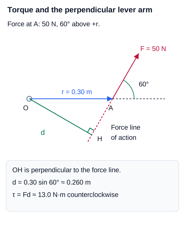
Wrench showing position vector, oblique force, and perpendicular lever arm — Torque and the Perpendicular Lever Arm
Only the component of force perpendicular to the position vector contributes to torque magnitude.

Moment of Inertia ( $I$ )

$I$

The rotational analog to mass, which measures an object's resistance to changes in its rotation. It depends on how the mass is distributed relative to the specific axis of rotation.

Moment of Inertia for Discrete Masses

Calculates moment of inertia for a system of point masses.

I = \sum m_i r_i^2

Variables

Symbol	Description	Unit
$I$	Moment of inertia	$kg\cdot m^2$
$m_i$	Mass of particle i	kg
$r_i$	Distance of particle i from axis	m

Moment of Inertia for Continuous Bodies

Calculates moment of inertia for a continuous solid body.

I = \int r^2 \, dm = \int \rho r^2 \, dV

Variables

Symbol	Description	Unit
$I$	Moment of inertia	$kg\cdot m^2$
$r$	Distance from axis	m
$dm$	Infinitesimal mass element	kg
$\rho$	Density of the body	$kg/m^3$
$dV$	Infinitesimal volume element	$m^3$

$Common Moments of Inertia$

Solid Cylinder or Disk (axis through center): $I = \frac{1}{2}MR^2$
Hoop or Thin Cylindrical Shell (axis through center): $I = MR^2$
Solid Sphere (axis through center): $I = \frac{2}{5}MR^2$
Thin Rod (axis through center): $I = \frac{1}{12}ML^2$
Thin Rod (axis through end): $I = \frac{1}{3}ML^2$

Parallel-Axis Theorem

Finds moment of inertia around an axis parallel to the center of mass axis.

I = I_{cm} + Md^2

Variables

Symbol	Description	Unit
$I$	Moment of inertia about parallel axis	$kg\cdot m^2$
$I_{cm}$	Moment of inertia about center of mass	$kg\cdot m^2$
$M$	Total mass	kg
$d$	Distance between parallel axes	m

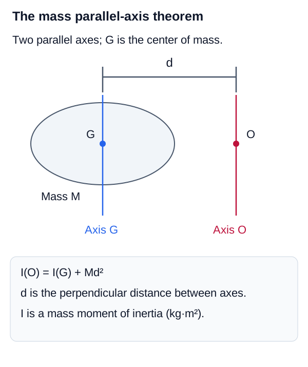
Body with centroidal axis and a parallel shifted axis separated by distance d — Parallel-Axis Geometry
Moving the reference axis a distance d from the center-of-mass axis adds Md squared to the moment of inertia.

$Interactive Simulation$

Use this inertia model to compare how mass distribution changes resistance to angular acceleration. Its radius control represents the same physical outer radius used in both the geometry and inertia equations.

Rotational Shape Profile

5 kg

1.2 m

15 N

Inertia Equation for Profile

I = \frac{1}{2} M R^2

A solid cylinder / disk has its mass evenly distributed from the center axle out to the radius R. More mass distributed far from the center yields a larger moment of inertia $I$ .

Moment of Inertia (I)

3.60 kg·m²

Applied Torque (τ = F·R)

18.00 N·m

Angular Accel. (α = τ/I)

5.00 rad/s²

Angular Velocity (ω)

0.00 rad/s

Newton's Second Law for Rotation

$Newton's Second Law for Rotation Concepts$

With torque and moment of inertia defined, we can state the rotational equivalent of $F=ma$ . The net torque on a rigid body is equal to its moment of inertia multiplied by its angular acceleration.

Newton's Second Law for Rotation

Relates net torque, moment of inertia, and angular acceleration.

\Sigma \vec{\tau} = I \vec{\alpha}

Variables

Symbol	Description	Unit
$\Sigma \vec{\tau}$	Net torque	$N\cdot m$
$I$	Moment of inertia	$kg\cdot m^2$
$\vec{\alpha}$	Angular acceleration vector	$rad/s^2$

Rotational Energy and Work

$Rotational Energy and Work Concepts$

A spinning object has kinetic energy, even if its center of mass is stationary.

$K_R$

The kinetic energy possessed by an object due to its rotational motion.

Rotational Kinetic Energy Equation

Calculates kinetic energy from rotational motion.

K_R = \frac{1}{2}I\omega^2

Variables

Symbol	Description	Unit
$K_R$	Rotational kinetic energy	J
$I$	Moment of inertia	$kg\cdot m^2$
$\omega$	Angular velocity	rad/s

Rolling Without Slipping

$Rolling Without Slipping Concepts$

When a wheel or sphere rolls across a surface without slipping, there is a strict relationship between its translational velocity ( $v_{cm}$ ) and its angular velocity ( $\omega$ ). Because it is both translating and rotating, its total kinetic energy is the sum of its translational and rotational kinetic energies: $K_{total} = \frac{1}{2}Mv_{cm}^2 + \frac{1}{2}I_{cm}\omega^2$ .

Rolling Translational Velocity

Relates center of mass velocity to angular velocity.

v_{cm} = R \omega

Variables

Symbol	Description	Unit
$v_{cm}$	Velocity of the center of mass	m/s
$R$	Radius of the rolling object	m
$\omega$	Angular velocity	rad/s

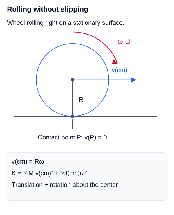
Wheel rolling without slipping with translational velocity, angular velocity, radius, and kinetic-energy partition — Rolling without Slipping and Energy Partition
For pure rolling, v at the center equals R omega, and total kinetic energy contains both translational and rotational terms.

$Work-Energy Theorem for Rotation$

The work done by a torque $\tau$ rotating an object through an angle $\Delta\theta$ is equal to the change in rotational kinetic energy.

Work Done by Torque

Calculates work done by applying torque over an angle.

W = \int \tau \, d\theta

Variables

Symbol	Description	Unit
$W$	Work done	J
$\tau$	Torque	$N\cdot m$
$d\theta$	Infinitesimal angular displacement	rad

Angular Momentum ( $L$ )

$\vec{L}$

The rotational analog to linear momentum ( $p=mv$ ). For a rigid body rotating about a fixed axis of symmetry, it is the product of moment of inertia and angular velocity.

Angular Momentum of a Point Particle

Angular momentum for a point particle relative to an origin.

\vec{L} = \vec{r} \times \vec{p}

Variables

Symbol	Description	Unit
$\vec{L}$	Angular momentum vector	$kg\cdot m^2/s$
$\vec{r}$	Position vector	m
$\vec{p}$	Linear momentum vector	$kg\cdot m/s$

Angular Momentum of a Rigid Body

Angular momentum for a rigid body rotating around a fixed axis.

\vec{L} = I\vec{\omega}

Variables

Symbol	Description	Unit
$\vec{L}$	Angular momentum vector	$kg\cdot m^2/s$
$I$	Moment of inertia	$kg\cdot m^2$
$\vec{\omega}$	Angular velocity vector	rad/s

$Conservation of Angular Momentum$

Just as $\Sigma F = dp/dt$ , the net torque equals the rate of change of angular momentum: $\Sigma \vec{\tau} = d\vec{L}/dt$ .

$Conservation Principle$

Conservation of Angular Momentum: If the net external torque on a system is zero ( $\Sigma \vec{\tau}_{ext} = 0$ ), the total angular momentum of the system is conserved ( $\vec{L}_i = \vec{L}_f$ ). This explains why a figure skater spins faster when they pull their arms in (decreasing $I$ must increase $\omega$ to keep $L=I\omega$ constant).

$Interactive Simulation$

Use this angular momentum model to see why pulling mass inward makes angular speed rise when external torque is negligible.

1.30 m

0.70 m

2.0 kg·m²

2.5 rad/s

Governing Laws

Moment of Inertia

I = I_{body} + 2m \cdot r^2

Conservation of Angular Momentum

L = I_i \cdot \omega_i = I_f \cdot \omega_f

Angular Momentum (L)

17.68 kg·m²/s

Current Angular Speed (ω)

5.09 rad/s

Initial Inertia (Iᵢ)

7.07 kg·m²

Current Inertia (I_c)

3.47 kg·m²

Parallel-Axis Theorem in Practice

$Calculating Complex Inertia$

The Parallel-Axis Theorem is not just an abstract concept; it is vital for calculating the moment of inertia of complex, composite engineering shapes (like I-beams or rotating eccentric cams) where the axis of rotation does not pass through the center of mass of every individual component.

By breaking a complex shape into simple geometric parts (rectangles, circles), finding their individual moments of inertia about their own centers of mass, and then using the Parallel-Axis Theorem ( $I = I_{cm} + Md^2$ ) to shift those moments to the global axis of rotation, engineers can analyze the rotational dynamics of virtually any rigid body.

Key Takeaways

Rotational kinematics equations ( $\theta, \omega, \alpha$ ) are exactly analogous to linear equations ( $x, v, a$ ).
Torque ( $\vec{\tau} = \vec{r} \times \vec{F}$ ) is the rotational analog to force, causing angular acceleration.
Moment of Inertia ( $I = \sum mr^2$ ) is the rotational analog to mass, representing resistance to angular acceleration. It depends on mass distribution.
Newton's Second Law for rotation is $\Sigma \vec{\tau} = I \vec{\alpha}$ .
A spinning object possesses Rotational Kinetic Energy ( $K_R = \frac{1}{2}I\omega^2$ ).
Angular Momentum ( $\vec{L} = I\vec{\omega}$ ) is conserved if the net external torque is zero.

$References$

Previous TopicImpulse and Momentum - Theory & Concepts

Quiz Me

Next TopicEquilibrium and Elasticity - Theory & Concepts

Prev Next

Quiz Me

Learning Objectives

Angular Kinematics

Angular Position (θ\thetaθ)

Angular Position Equation

Angular Velocity (ω\omegaω)

Angular Velocity Equations

Angular Acceleration (α\alphaα)

Angular Acceleration Equations

The Analogies

The Analogies Concepts

Kinematic Analogies

Right-Hand Rule

Interactive Simulation

Rotational Dynamics

Rotational Dynamics Concepts

Torque (τ⃗\vec{\tau}τ)

Torque Equation

Torque Magnitude Equation

Moment of Inertia (III)

Moment of Inertia (III)

Moment of Inertia for Discrete Masses

Moment of Inertia for Continuous Bodies

Common Moments of Inertia

Parallel-Axis Theorem

Interactive Simulation

Newton's Second Law for Rotation

Newton's Second Law for Rotation Concepts

Newton's Second Law for Rotation

Rotational Energy and Work

Rotational Energy and Work Concepts

Rotational Kinetic Energy (KRK_RKR​)

Rotational Kinetic Energy Equation

Rolling Without Slipping

Rolling Without Slipping Concepts

Rolling Translational Velocity

Work-Energy Theorem for Rotation

Work Done by Torque

Angular Momentum (LLL)

Angular Momentum (L⃗\vec{L}L)

Angular Momentum of a Point Particle

Angular Momentum of a Rigid Body

Conservation of Angular Momentum

Conservation Principle

Interactive Simulation

Parallel-Axis Theorem in Practice

Calculating Complex Inertia

References

$Learning Objectives$

$\theta$

$\omega$

$\alpha$

$The Analogies Concepts$

$Kinematic Analogies$

$Right-Hand Rule$

$Interactive Simulation$

$Rotational Dynamics Concepts$

$\vec{\tau}$

Moment of Inertia ( $I$ )

$I$

$Common Moments of Inertia$

$Interactive Simulation$

$Newton's Second Law for Rotation Concepts$

$Rotational Energy and Work Concepts$

$K_R$

$Rolling Without Slipping Concepts$

$Work-Energy Theorem for Rotation$

Angular Momentum ( $L$ )

$\vec{L}$

$Conservation of Angular Momentum$

$Conservation Principle$

$Interactive Simulation$

$Calculating Complex Inertia$

$References$