Impulse and Momentum

Impulse and Momentum

$Learning Objectives$

Define linear momentum and impulse as vector quantities.
Apply the Impulse-Momentum Theorem to solve for force, time, or velocity changes.
State and apply the principle of Conservation of Linear Momentum.
Analyze 1D and 2D collisions, distinguishing between elastic, inelastic, and perfectly inelastic collisions.
Use the coefficient of restitution to quantify the elasticity of collisions.
Analyze variable mass systems using the Tsiolkovsky rocket equation.

In mechanics, understanding how forces act over time is crucial for analyzing impacts, crashes, and explosions. This is the realm of impulse and momentum. While the Work-Energy theorem deals with forces acting over a distance, the Impulse-Momentum theorem deals with forces acting over time. This distinction is critical because in many real-world scenarios—like a car crash, a hammer striking a nail, or a jet engine providing thrust—the force is not constant and acts over a very short duration. We cannot easily measure the force or the distance during the impact, but we can measure the velocities before and after.

Center of Mass Frame

$Center of Mass Frame Concepts$

Before analyzing collisions, it is helpful to define the center of mass (CM) velocity. For a system of particles, the CM moves with a constant velocity if no external forces act on the system.

Center of Mass Velocity

Calculates the velocity of the center of mass for a system of particles.

\vec{v}_{cm} = \frac{\Sigma m_i \vec{v}_i}{\Sigma m_i} = \frac{\vec{P}_{total}}{M_{total}}

Variables

Symbol	Description	Unit
$\vec{v}_{cm}$	Center of mass velocity	$\text{m/s}$
$m_i$	Mass of individual particle	kg
$\vec{v}_i$	Velocity of individual particle	$\text{m/s}$
$\vec{P}_{total}$	Total momentum of the system	$\text{kg} \cdot \text{m/s}$
$M_{total}$	Total mass of the system	kg

$Center of Mass Frame Concepts$

In the CM reference frame, the total momentum of the system is always identically zero. This makes analyzing complex collisions (especially in 2D or 3D) mathematically much simpler.

Linear Momentum ( $p$ )

$p$

Momentum is a measure of "how hard it is to stop" an object. It depends on both how massive the object is and how fast it's moving.

$\vec{p}$

The product of an object's mass and its velocity. It is a vector quantity, pointing in the same direction as the velocity. The SI unit is $\text{kg} \cdot \text{m/s}$ .

Linear Momentum

Calculates the linear momentum of an object.

\vec{p} = m\vec{v}

Variables

Symbol	Description	Unit
$\vec{p}$	Linear momentum vector	$\text{kg} \cdot \text{m/s}$
$m$	Mass of the object	kg
$\vec{v}$	Velocity vector	$\text{m/s}$

$p$

Newton actually formulated his Second Law in terms of momentum, not acceleration. The net force on an object is equal to the rate of change of its momentum.

Newton's Second Law in terms of Momentum

Expresses the net force as the rate of change of momentum.

\Sigma \vec{F} = \frac{d\vec{p}}{dt} = \frac{d(m\vec{v})}{dt}

Variables

Symbol	Description	Unit
$\Sigma \vec{F}$	Net force vector	N
$\vec{p}$	Momentum vector	$\text{kg} \cdot \text{m/s}$
$t$	Time	s
$m$	Mass	kg
$\vec{v}$	Velocity vector	$\text{m/s}$

$p$

If mass is constant, this simplifies to our familiar $F=ma$ . However, this general form is powerful because it allows us to analyze systems where mass is changing, like a rocket burning fuel.

Impulse ( $J$ )

$J$

If momentum is the "amount of motion," then impulse is the "change in motion" caused by a force acting over a time interval.

$\vec{J}$

The integral of a force over the time interval during which it acts. It is a vector quantity, pointing in the same direction as the force. The SI unit is $\text{N} \cdot \text{s}$ (which is equivalent to $\text{kg} \cdot \text{m/s}$ ).

Impulse

Calculates the impulse delivered by a variable or constant force.

\vec{J} = \int_{t_i}^{t_f} \vec{F}(t) \, dt

\vec{J} = \vec{F}_{avg} \Delta t

Variables

Symbol	Description	Unit
$\vec{J}$	Impulse vector	$\text{N} \cdot \text{s}$
$\vec{F}(t)$	Force as a function of time	N
$t_i$	Initial time	s
$t_f$	Final time	s
$\vec{F}_{avg}$	Average force	N
$\Delta t$	Time interval	s

$J$

For a constant force, the calculation simplifies to multiplying the average force by the time interval.

$J$

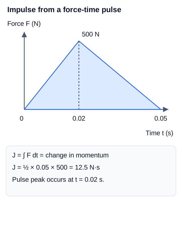
Graphically, impulse is the area under a Force vs. Time curve. This is why airbags and crumple zones save lives in car crashes. They increase the time ( $\Delta t$ ) over which a passenger's momentum is reduced to zero. By increasing the time, the average force ( $\vec{F}_{avg}$ ) required to deliver the necessary impulse ( $\vec{J}$ ) decreases significantly.

$Interactive Simulation: Impulse and Momentum$

Use this impulse model to see how the same change in momentum can be produced by different force-time combinations.

Idealized Force Pulse

900 N

0.18 s

3.0 kg

0.65

Governing Relations

Impulse-Momentum Theorem

J(t)=\int_0^t F(\tau)\,d\tau=m\,\Delta v(t)

Total Pulse Impulse

J=\tfrac12F_{peak}\Delta t

Current Force

630.0 N

Current Impulse J(t)

61.2 N·s

Current Δv

20.39 m/s

Final Δv

27.00 m/s

Cart translation is a schematic time-progress indicator; the quantitative teaching result is the force-time area and the corresponding momentum change.

Triangular force-time pulse whose shaded area represents impulse — Impulse as Area under a Force-Time Curve
The area under a force-time history is the impulse. A longer stopping interval can reduce average force for the same momentum change.

The Impulse-Momentum Theorem

$The Impulse-Momentum Theorem Concepts$

Just as the Work-Energy theorem connects work and kinetic energy, the Impulse-Momentum theorem connects impulse and momentum.

$The Impulse-Momentum Theorem$

The net impulse exerted on a particle is equal to the change in the particle's momentum.

The Impulse-Momentum Theorem

Relates the net impulse applied to an object to its change in momentum.

\vec{J}_{net} = \Delta \vec{p} = \vec{p}_f - \vec{p}_i = m\vec{v}_f - m\vec{v}_i

Variables

Symbol	Description	Unit
$\vec{J}_{net}$	Net impulse vector	$\text{N} \cdot \text{s}$
$\Delta \vec{p}$	Change in momentum vector	$\text{kg} \cdot \text{m/s}$
$\vec{p}_f$	Final momentum vector	$\text{kg} \cdot \text{m/s}$
$\vec{p}_i$	Initial momentum vector	$\text{kg} \cdot \text{m/s}$
$m$	Mass	kg
$\vec{v}_f$	Final velocity vector	$\text{m/s}$
$\vec{v}_i$	Initial velocity vector	$\text{m/s}$

$The Impulse-Momentum Theorem Concepts$

This theorem is essentially Newton's Second Law rewritten to focus on the time interval over which a force acts.

Conservation of Linear Momentum

$Conservation of Linear Momentum Concepts$

The true power of momentum lies in analyzing systems of interacting particles. When two objects collide, the forces they exert on each other are internal to the system. By Newton's Third Law, these forces are equal and opposite, so the impulses they impart to each other are also equal and opposite ( $\vec{J}_{1 \text{ on } 2} = -\vec{J}_{2 \text{ on } 1}$ ).

This leads to a profound conclusion.

$Conservation of Linear Momentum$

If the net external force on a system is zero ( $\Sigma \vec{F}_{ext} = 0$ ), then the total linear momentum of the system is conserved (remains constant).

Conservation of Linear Momentum

States that total momentum before a collision equals total momentum after a collision for a closed system.

\vec{P}_{total, i} = \vec{P}_{total, f}

m_1\vec{v}_{1i} + m_2\vec{v}_{2i} = m_1\vec{v}_{1f} + m_2\vec{v}_{2f}

Variables

Symbol	Description	Unit
$\vec{P}_{total}$	Total momentum vector	$\text{kg} \cdot \text{m/s}$
$m_1, m_2$	Masses of interacting objects	kg
$\vec{v}_{1i}, \vec{v}_{2i}$	Initial velocity vectors	$\text{m/s}$
$\vec{v}_{1f}, \vec{v}_{2f}$	Final velocity vectors	$\text{m/s}$
$i, f$	Initial and final states	-

$Vector Conservation of Momentum$

Momentum is a vector quantity. This means momentum must be conserved in each spatial dimension independently. In a 2D collision on an x-y plane:

\begin{aligned} \Sigma p_{xi} &= \Sigma p_{xf} \\ \Sigma p_{yi} &= \Sigma p_{yf} \end{aligned}

$Interactive Simulation: Collision Momentum$

Use this smooth-contact planar collision model to resolve velocity into normal and tangential components. The simulation conserves momentum in both Cartesian directions and applies restitution only along the line of impact.

Closing impact

Body A

2.0 kg

6.00 m/s

10 °

Body B

3.0 kg

2.00 m/s

190 °

0 °

0.50

Normal / tangential decomposition

A: uₙ = 5.91 m/s, uₜ = 1.04 m/s

B: uₙ = -1.97 m/s, uₜ = -0.35 m/s

pₓ before → after

5.91 → 5.91 kg·m/s

pᵧ before → after

1.04 → 1.04 kg·m/s

Restitution check

0.500

Kinetic-energy loss

27.93 J

Momentum residual

8.88e-16 kg·m/s

Relative normal approach

7.88 m/s

Center-of-mass frame

COM velocity = (1.18, 0.21) m/s. The total momentum in this frame is zero before and after impact.

A: (4.73, 0.83) → (-2.36, 0.83) m/s

B: (-3.15, -0.56) → (1.58, -0.56) m/s

Circle size is schematic and does not encode mass. The selected line of impact determines the contact-normal direction.

Variable Mass Systems: Rocket Equation

$Variable Mass Systems: Rocket Equation Concepts$

A classic application of the generalized Newton's Second Law ( $\Sigma \vec{F} = \frac{d\vec{p}}{dt}$ ) is analyzing systems where mass is continuously ejected or accumulated, such as a rocket.

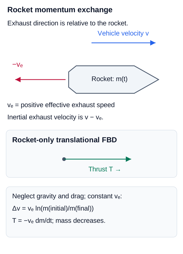
A rocket accelerates by ejecting mass (exhaust gas) backwards at a high relative velocity ( $v_e$ ). Conservation of momentum gives the Tsiolkovsky rocket equation, which relates the change in velocity ( $\Delta v$ ) to the effective exhaust velocity ( $v_e$ ) and the initial ( $m_i$ ) and final ( $m_f$ ) mass of the rocket:

Tsiolkovsky Rocket Equation

Calculates the change in velocity of a rocket based on its exhaust velocity and mass ratio.

\Delta v = v_e \ln\left(\frac{m_i}{m_f}\right)

Variables

Symbol	Description	Unit
$\Delta v$	Change in velocity	$\text{m/s}$
$v_e$	Effective exhaust velocity	$\text{m/s}$
$m_i$	Initial mass (including fuel)	kg
$m_f$	Final mass (after fuel is burned)	kg

$Variable Mass Systems: Rocket Equation Concepts$

For the ideal momentum-only rocket model, the thrust magnitude is commonly written $T=\dot{m}v_e$ , where $\dot{m}$ is the positive exhaust mass-flow rate. A real rocket's complete thrust expression can also include a nozzle pressure term, so the ideal rocket equation must not be interpreted as a complete launch-trajectory model.

Rocket moving forward while exhaust mass is expelled backward at an effective relative exhaust speed — Variable-Mass Momentum Exchange
The rocket gains forward momentum as propellant mass is ejected backward. The ideal velocity increment depends logarithmically on mass ratio.

Types of Collisions

$Types of Collisions Concepts$

While total momentum is always conserved in a collision (if external forces are negligible), kinetic energy is not necessarily conserved. Collisions are classified by what happens to the total kinetic energy.

Elastic Collisions: Both momentum and total kinetic energy are conserved. The objects bounce off each other perfectly without any loss of mechanical energy to heat or deformation. Example: Billiard balls (approximately), gas molecules.
Inelastic Collisions: Momentum is conserved, but kinetic energy is not. Some kinetic energy is converted into internal energy (heat, sound, deformation). Most real-world macroscopic collisions are inelastic.
Perfectly Inelastic Collisions: A specific type of inelastic collision where the objects stick together and move with a common final velocity after the impact. This results in the maximum possible loss of kinetic energy (though momentum is still conserved).

Coefficient of Restitution ( $e$ )

$e$

The degree of elasticity in a 1D collision is quantified by the coefficient of restitution, $e$ . It relates the relative speeds of approach and separation.

$e$

The ratio of the relative speed of separation after collision to the relative speed of approach before collision.

Coefficient of Restitution

Quantifies the elasticity of a 1D collision.

e = \frac{v_{2f} - v_{1f}}{v_{1i} - v_{2i}}

Variables

Symbol	Description	Unit
$e$	Coefficient of restitution	-
$v_{1i}, v_{2i}$	Initial velocities	$\text{m/s}$
$v_{1f}, v_{2f}$	Final velocities	$\text{m/s}$

$e$

$e = 1$ $e = 1$ : Perfectly elastic collision.
- $0 < e < 1$ : Inelastic collision.
- $e = 0$ : Perfectly inelastic collision (objects stick together, $v_{1f} = v_{2f}$ ).

Collisions in Two Dimensions

$Vector Conservation$

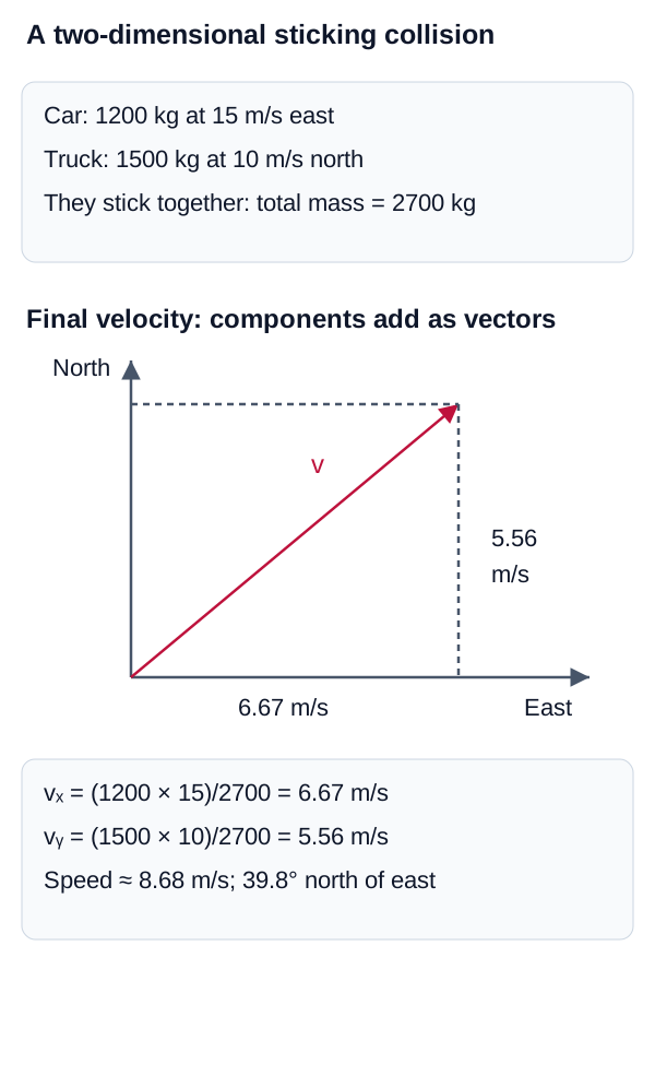
In two-dimensional collisions, such as a glancing blow in billiards or a vehicle intersection crash, momentum is conserved independently in both the $x$ and $y$ directions. The principles are the same as 1D collisions, but require the use of vector components.

2D Momentum Conservation Equations

The separated x and y component equations for conservation of linear momentum.

\begin{aligned} \sum p_{xi} &= \sum p_{xf} \implies m_1 v_{1ix} + m_2 v_{2ix} = m_1 v_{1fx} + m_2 v_{2fx} \\ \sum p_{yi} &= \sum p_{yf} \implies m_1 v_{1iy} + m_2 v_{2iy} = m_1 v_{1fy} + m_2 v_{2fy} \end{aligned}

Variables

Symbol	Description	Unit
$p_{x}$	Momentum in x-direction	$\text{kg} \cdot \text{m/s}$
$p_{y}$	Momentum in y-direction	$\text{kg} \cdot \text{m/s}$

$Restitution Along the Line of Impact$

For a smooth two-body impact, resolve each velocity into a component normal to the contact plane (along the line of impact) and a tangential component. The contact impulse acts along the normal direction, so the tangential components remain unchanged. The model must only be applied when the pre-impact normal relative velocity is closing.

Normal Restitution Relation

Relates the normal relative separation speed to the normal relative approach speed for a smooth impact.

e = \frac{v_{2n,f}-v_{1n,f}}{v_{1n,i}-v_{2n,i}}

Variables

Symbol	Description	Unit
$e$	Coefficient of restitution	dimensionless
$v_{1n,i}, v_{2n,i}$	Initial normal velocity components	m/s
$v_{1n,f}, v_{2n,f}$	Final normal velocity components	m/s

Two perpendicular vehicle momentum vectors combining into a two-dimensional final momentum vector — Two-Dimensional Momentum Components
Momentum is conserved independently in the x and y directions; a vector result cannot be replaced by a one-dimensional scalar balance.

Key Takeaways

Momentum ( $\vec{p} = m\vec{v}$ ) is a vector describing the "amount of motion." The net force equals the rate of change of momentum.
Impulse ( $\vec{J} = \int \vec{F} dt$ ) is a vector describing the "change in motion." It equals the change in momentum ( $\vec{J} = \Delta\vec{p}$ ).
The Conservation of Momentum principle states that the total momentum of a system is constant if no net external forces act on it.
In Elastic collisions, both momentum and kinetic energy are conserved. In Inelastic collisions, only momentum is conserved; kinetic energy is lost. The Coefficient of Restitution quantifies this.

$References$

Previous TopicWork, Energy, and Power - Theory & Concepts

Quiz Me

Next TopicRotational Motion - Theory & Concepts

Prev Next

Quiz Me

Learning Objectives

Center of Mass Frame

Center of Mass Frame Concepts

Center of Mass Velocity

Center of Mass Frame Concepts

Linear Momentum (ppp)

Linear Momentum (ppp) Concepts

Linear Momentum (p⃗\vec{p}p​)

Linear Momentum

Linear Momentum (ppp) Concepts

Newton's Second Law in terms of Momentum

Linear Momentum (ppp) Concepts

Impulse (JJJ)

Impulse (JJJ) Concepts

Impulse (J⃗\vec{J}J)

Impulse

Impulse (JJJ) Concepts

Impulse (JJJ) Concepts

Interactive Simulation: Impulse and Momentum

The Impulse-Momentum Theorem

The Impulse-Momentum Theorem Concepts

The Impulse-Momentum Theorem

The Impulse-Momentum Theorem

The Impulse-Momentum Theorem Concepts

Conservation of Linear Momentum

Conservation of Linear Momentum Concepts

Conservation of Linear Momentum

Conservation of Linear Momentum

Vector Conservation of Momentum

Interactive Simulation: Collision Momentum

Variable Mass Systems: Rocket Equation

Variable Mass Systems: Rocket Equation Concepts

Tsiolkovsky Rocket Equation

Variable Mass Systems: Rocket Equation Concepts

Types of Collisions

Types of Collisions Concepts

Coefficient of Restitution (eee)

Coefficient of Restitution (eee) Concepts

Coefficient of Restitution (eee)

Coefficient of Restitution

Coefficient of Restitution (eee) Concepts

Collisions in Two Dimensions

Vector Conservation

2D Momentum Conservation Equations

Restitution Along the Line of Impact

Normal Restitution Relation

References

$Learning Objectives$

$Center of Mass Frame Concepts$

$Center of Mass Frame Concepts$

Linear Momentum ( $p$ )

$p$

$\vec{p}$

$p$

$p$

Impulse ( $J$ )

$J$

$\vec{J}$

$J$

$J$

$Interactive Simulation: Impulse and Momentum$

$The Impulse-Momentum Theorem Concepts$

$The Impulse-Momentum Theorem$

$The Impulse-Momentum Theorem Concepts$

$Conservation of Linear Momentum Concepts$

$Conservation of Linear Momentum$

$Vector Conservation of Momentum$

$Interactive Simulation: Collision Momentum$

$Variable Mass Systems: Rocket Equation Concepts$

$Variable Mass Systems: Rocket Equation Concepts$

$Types of Collisions Concepts$

Coefficient of Restitution ( $e$ )

$e$

$e$

$e$

$Vector Conservation$

$Restitution Along the Line of Impact$

$References$