Electricity and Magnetism

Electricity and Magnetism

$Learning Objectives$

Define electric charge and apply Coulomb's Law.
Understand the concept of electric fields and apply Gauss's Law.
Calculate electric potential and capacitance.
Analyze simple DC circuits using Ohm's Law and Kirchhoff's Rules.
Describe magnetic fields, the magnetic force on moving charges, and sources of magnetic fields.
Explain electromagnetic induction using Faraday's Law and Lenz's Law.

Electricity and Magnetism (Electromagnetism) govern the interactions between electrically charged particles. This field is foundational for electrical engineering, power transmission, and electronics.

Electric Charge

$Electric Charge Concepts$

Matter is composed of atoms, which contain positively charged protons and negatively charged electrons. The fundamental unit of charge ( $e$ ) is $1.602 \times 10^{-19}$ Coulombs (C).

Protons: $+e$
Electrons: $-e$

Charge ( $q$ ) is a conserved property. The total charge of an isolated system remains constant. Like charges repel; opposite charges attract.

Coulomb's Law

$Coulomb's Law Concepts$

The fundamental force between two point charges ( $q_1$ and $q_2$ ) separated by a distance ( $r$ ) is given by Coulomb's Law. It is mathematically identical in form to Newton's Law of Universal Gravitation, but the force can be attractive or repulsive.

Coulomb Force Magnitude

Magnitude of the electrostatic force between two stationary point charges in vacuum.

F = k \frac{|q_1 q_2|}{r^2} = \frac{1}{4\pi\epsilon_0}\frac{|q_1 q_2|}{r^2}

Variables

Symbol	Description	Unit
$F$	Electrostatic force magnitude	N
$q_1$	First point charge	C
$q_2$	Second point charge	C
$r$	Separation between charges	m
$k$	Coulomb constant	$N·m^2/C^2$
$\epsilon_0$	Vacuum permittivity	F/m

$Interactive Simulation$

Use this electric force model to see how charge signs, magnitudes, and separation control attraction or repulsion.

Attracts

5 μC

-5 μC

10 cm

Governing Formula

F = k_e \cdot \frac{|q_1 \cdot q_2|}{r^2}

Where electrostatic constant $k_e \approx 8.99 \times 10^9 \text{ N}\cdot\text{m}^2/\text{C}^2$. Force is proportional to charge product and inversely proportional to $r^2$.

Force magnitude (F)

22.47 N

Interaction Type

Attractive

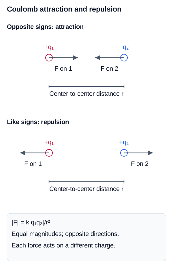
Two point charges with equal and opposite Coulomb force vectors, separation r, and attraction and repulsion direction cases. — Two-Charge Coulomb Force Geometry
The force pair is equal in magnitude and opposite in direction; its sense changes from attraction to repulsion with the charge signs, while magnitude follows the inverse-square distance law.

The Electric Field ( $\vec{E}$ )

$\vec{E}$

Instead of thinking of charges exerting forces directly on one another across empty space, we introduce the concept of an electric field. A charge creates an electric field in the space around it, and another charge placed in that field feels a force.

$\vec{E}$

The electrostatic force per unit charge exerted on a positive test charge ( $q_0$ ) at a specific point in space. Electric field lines point away from positive charges and towards negative charges.

Electric Field

Calculates the electric field at a point.

\vec{E} = \frac{\vec{F}}{q_0}

Variables

Symbol	Description	Unit
$\vec{E}$	Electric field	N/C or V/m
$\vec{F}$	Electrostatic force	N
$q_0$	Positive test charge	C

Electric Field of a Point Charge

Calculates the electric field created by a single point charge.

\vec{E} = k \frac{q}{r^2} \hat{r}

Variables

Symbol	Description	Unit
$\vec{E}$	Electric field	N/C or V/m
$k$	Coulomb's constant	$N\cdot m^2/C^2$
$q$	Point charge	C
$r$	Distance from the charge	m
$\hat{r}$	Unit vector pointing radially outward from the charge	dimensionless

Gauss's Law

$Gauss's Law Concepts$

Gauss's Law is a powerful alternative to Coulomb's law for calculating electric fields of symmetric charge distributions (like spheres, cylinders, or infinite planes). It relates the electric flux ( $\Phi_E$ ) passing through a closed "Gaussian" surface to the total charge enclosed within that surface ( $q_{enc}$ ).

Gauss's Law

Relates the electric flux passing through a closed surface to the charge enclosed within it.

\Phi_E = \oint \vec{E} \cdot d\vec{A} = \frac{q_{enc}}{\epsilon_0}

Variables

Symbol	Description	Unit
$\Phi_E$	Electric flux	$V\cdot m$
$\vec{E}$	Electric field	N/C or V/m
$d\vec{A}$	Differential area vector	$m^2$
$q_{enc}$	Total enclosed charge	C
$\epsilon_0$	Permittivity of free space	$C^2/(N\cdot m^2)$

Electric Potential ( $V$ )

$V$

Just as a mass in a gravitational field has gravitational potential energy, a charge in an electric field has electric potential energy ( $U$ ). Because the electrostatic force is conservative, we can define a potential energy function.

It is often more useful to talk about energy per unit charge, which is the electric potential (commonly called Voltage).

$V$

The electric potential energy per unit charge at a point in an electric field. The SI unit is the Volt (V), where $1 \text{ V} = 1 \text{ J/C}$ .

Electric Potential

Calculates the electric potential energy per unit charge.

V = \frac{U}{q}

Variables

Symbol	Description	Unit
$V$	Electric potential	V
$U$	Electric potential energy	J
$q$	Charge	C

Electric Potential of a Point Charge

Calculates the electric potential created by a single point charge.

V = k \frac{q}{r}

Variables

Symbol	Description	Unit
$V$	Electric potential	V
$k$	Coulomb's constant	$N\cdot m^2/C^2$
$q$	Point charge	C
$r$	Distance from the charge	m

$V$

The difference in potential between two points ( $\Delta V$ ) is the voltage. It represents the work done per unit charge by an external agent moving a positive test charge between those points.

Voltage (Potential Difference)

Calculates the difference in electric potential between two points.

\Delta V = V_f - V_i = \frac{\Delta U}{q} = - \int \vec{E} \cdot d\vec{s}

Variables

Symbol	Description	Unit
$\Delta V$	Voltage or potential difference	V
$V_f, V_i$	Final and initial electric potentials	V
$\Delta U$	Change in electric potential energy	J
$q$	Charge	C
$\vec{E}$	Electric field	V/m
$d\vec{s}$	Differential path element	m

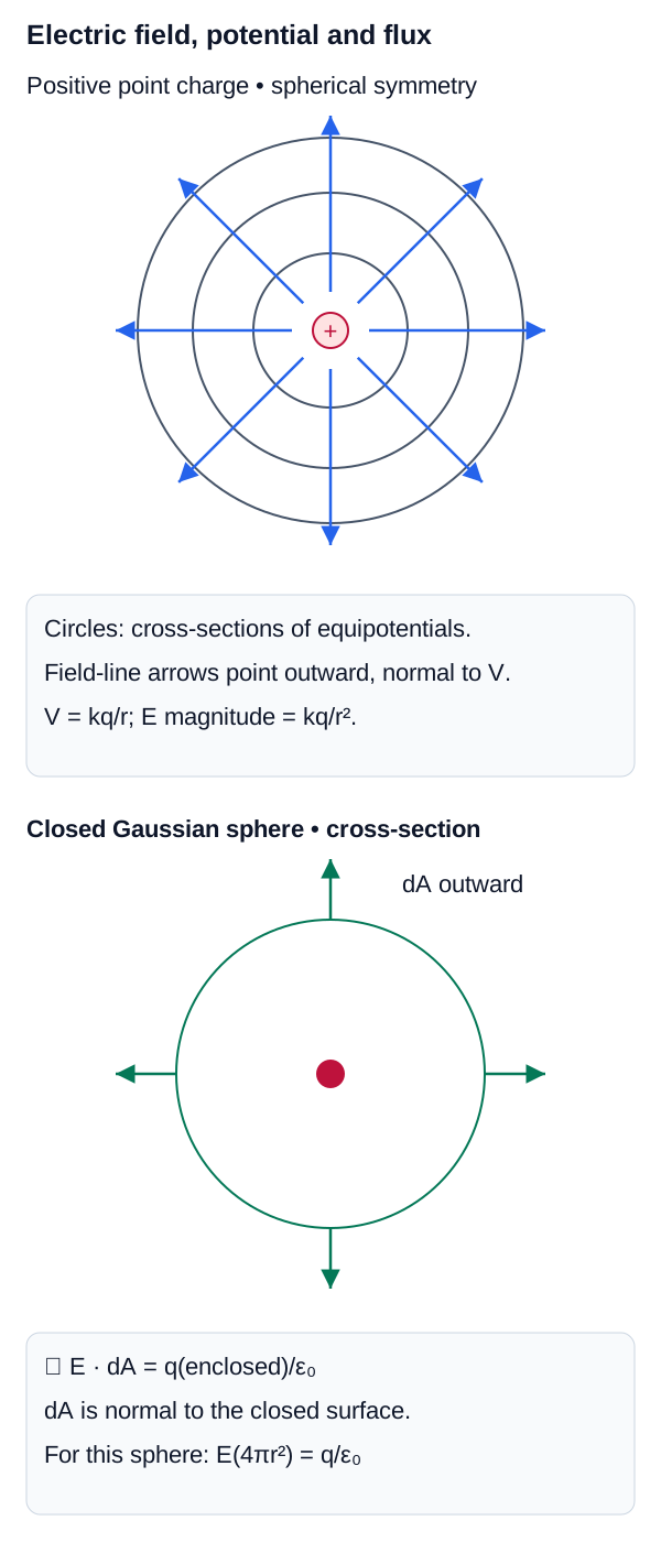
Electric field vectors around a positive charge, concentric equipotential contours, and a closed Gaussian surface with outward area vectors. — Electric Field, Equipotential, and Gaussian Surface
Field vectors are normal to equipotential contours, and Gauss's law relates net electric flux through a closed surface to enclosed charge.

Capacitance ( $C$ )

$C$

A capacitor is a device (usually two conducting plates separated by an insulator) that stores electric charge and potential energy.

$C$

The ratio of the magnitude of charge on either plate ( $Q$ ) to the potential difference ( $\Delta V$ ) between them. The SI unit is the Farad (F), where $1 \text{ F} = 1 \text{ C/V}$ .

Capacitance

Calculates the capacitance of a device.

C = \frac{Q}{\Delta V}

Variables

Symbol	Description	Unit
$C$	Capacitance	F
$Q$	Magnitude of charge on either plate	C
$\Delta V$	Potential difference between plates	V

Ideal Vacuum Parallel-Plate Capacitor

Capacitance of two large parallel plates separated by vacuum, neglecting edge fringing.

C = \epsilon_0 \frac{A}{d}

Variables

Symbol	Description	Unit
$C$	Capacitance	F
$\epsilon_0$	Permittivity of free space	$F/m or C^2/(N\cdot m^2)$
$A$	Area of each plate	$m^2$
$d$	Separation distance between plates	m

$C$

The energy stored in a capacitor is $U = \frac{1}{2} C (\Delta V)^2$ .

Current and Resistance

$Current and Resistance Concepts$

When charges move continuously, they form an electric current.

$I$

The rate of flow of electric charge through a cross-sectional area. The SI unit is the Ampere (A), where $1 \text{ A} = 1 \text{ C/s}$ .

Electric Current

Calculates the rate of charge flow.

I = \frac{dq}{dt}

Variables

Symbol	Description	Unit
$I$	Current	A
$dq$	Differential amount of charge	C
$dt$	Differential time interval	s

$Current and Resistance Concepts$

By convention, the direction of current is the direction positive charges would flow (opposite to the actual flow of electrons).

To drive a current through a conductor, a potential difference ( $\Delta V$ ) is required. Most materials resist this flow.

Ohm's Law

Relates current, voltage, and resistance for ohmic materials.

I = \frac{\Delta V}{R}

Variables

Symbol	Description	Unit
$I$	Current	A
$\Delta V$	Potential difference or voltage	V
$R$	Resistance	$\Omega$

$Interactive Simulation$

Switch between two-resistor series and parallel networks. The simulator reports equivalent resistance, total current, individual branch currents, voltage drops, and power from one circuit model.

12 V

6 Ω

4 Ω

R_{eq}=R_1+R_2,\quad I_1=I_2=I_T

Equivalent R

10.00 Ω

Total current

1.20 A

Total power

14.40 W

Branch I1

1.20 A

Branch I2

1.20 A

Power check

14.40 W

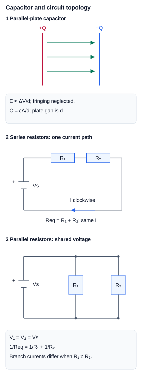
Parallel-plate capacitor field geometry and two-resistor series and parallel DC circuit schematics with current and voltage relationships. — Capacitor and Series–Parallel Circuit Geometry
The capacitor panel shows nearly uniform interior field in the ideal plate model; the circuit panels distinguish equal current in series from equal branch voltage in parallel.

$Current and Resistance Concepts$

Resistance depends on the material's resistivity ( $\rho$ ) and geometry: $R = \rho L / A$ .

The rate at which energy is dissipated in a resistor (power) is $P = I \Delta V = I^2 R = (\Delta V)^2 / R$ .

Kirchhoff's Rules

$Kirchhoff's Rules Concepts$

For analyzing complex circuits, we use two rules based on conservation laws:

Junction Rule (Conservation of Charge): The sum of currents entering any junction must equal the sum of currents leaving that junction ( $\Sigma I_{in} = \Sigma I_{out}$ ).
Loop Rule (Conservation of Energy): The algebraic sum of changes in potential around any closed circuit path (loop) must be zero ( $\Sigma \Delta V = 0$ ).

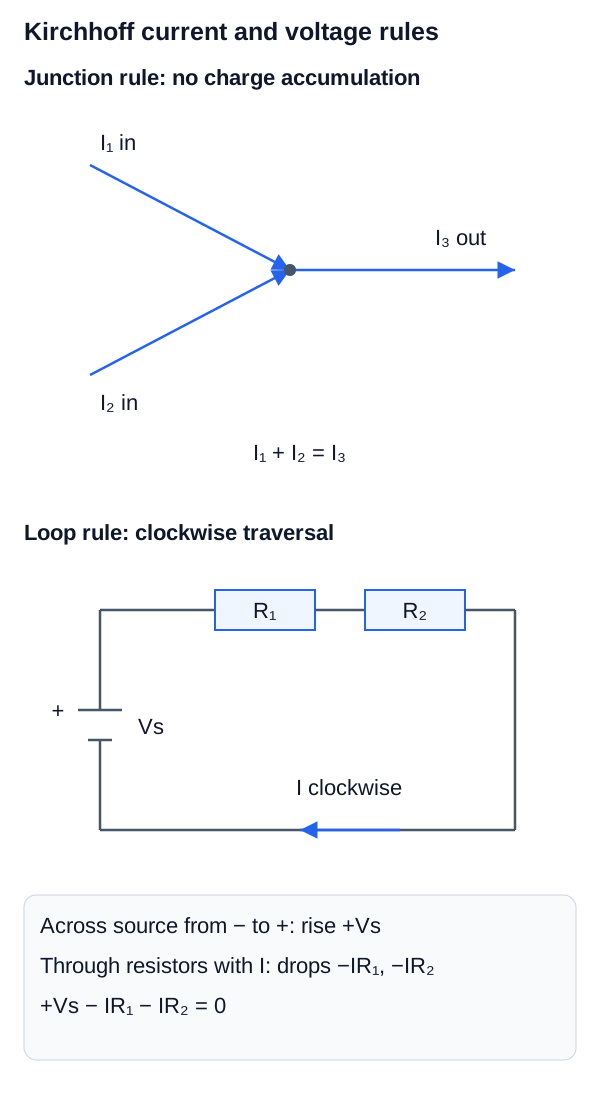
Circuit junction with labeled entering and leaving currents and a closed loop with voltage-rise and resistor-drop arrows. — Kirchhoff Junction and Loop Rules
The junction panel enforces charge conservation, while the loop panel tracks signed potential changes around a closed path.

Magnetism

$Magnetism Concepts$

Moving charges (currents) create magnetic fields ( $\vec{B}$ ). Magnetic fields, in turn, exert forces on moving charges.

$\vec{F}_B$

The force exerted by a magnetic field $\vec{B}$ on a charge $q$ moving with velocity $\vec{v}$ . The direction is determined by the Right-Hand Rule.

Magnetic Force

Calculates the force exerted by a magnetic field on a moving charge.

\vec{F}_B = q(\vec{v} \times \vec{B})

Variables

Symbol	Description	Unit
$\vec{F}_B$	Magnetic force	N
$q$	Charge	C
$\vec{v}$	Velocity vector	m/s
$\vec{B}$	Magnetic field vector	T

Magnetic Force on a Current-Carrying Segment

Force on a straight current-carrying segment in a uniform magnetic field.

\vec{F}_B = I(\vec{L}\times\vec{B}), \qquad F_B = I L B\sin\theta

Variables

Symbol	Description	Unit
$\vec{F}_B$	Magnetic force on the segment	N
$I$	Conventional current	A
$\vec{L}$	Length vector pointing in the current direction	m
$\vec{B}$	Magnetic field	T
$\theta$	Angle between current direction and magnetic field	$rad or ^\circ$

$Work and Magnetic Force$

Notice that the force is always perpendicular to both the velocity and the magnetic field. Therefore, a magnetic field can change the direction of a moving charge but cannot do work on it (cannot change its kinetic energy).

Sources of Magnetic Fields

$Sources of Magnetic Fields Concepts$

Magnetic fields are created by currents. The Biot-Savart Law and Ampere's Law allow us to calculate these fields. For highly symmetric current distributions, Ampere's Law is especially useful.

Magnetic Field of a Long Straight Wire

Calculates the magnetic field magnitude at a distance r from a long, straight current-carrying wire.

B = \frac{\mu_0 I}{2\pi r}

Variables

Symbol	Description	Unit
$B$	Magnetic field magnitude	T
$\mu_0$	Permeability of free space	$4\pi \times 10^{-7} \text{ T}\cdot\text{m/A}$
$I$	Current in the wire	A
$r$	Perpendicular distance from the wire	m

Magnetic Field at the Center of a Circular Loop

Calculates the magnetic field magnitude at the center of a single circular current loop.

B = \frac{\mu_0 I}{2R}

Variables

Symbol	Description	Unit
$B$	Magnetic field magnitude	T
$\mu_0$	Permeability of free space	$4\pi \times 10^{-7} \text{ T}\cdot\text{m/A}$
$I$	Current in the wire loop	A
$R$	Radius of the circular loop	m

Magnetic Field Inside a Long Solenoid

Calculates the nearly uniform magnetic field inside a long coil of wire.

B = \mu_0 n I

Variables

Symbol	Description	Unit
$B$	Magnetic field magnitude	T
$\mu_0$	Permeability of free space	$4\pi \times 10^{-7} \text{ T}\cdot\text{m/A}$
$n$	Number of turns per unit length (N/L)	1/m
$I$	Current in the wire	A

$Applications of Magnetism$

Electric Motors: Using magnetic forces on current-carrying loops to generate torque.
Transformers: Utilizing electromagnetic induction to step-up or step-down AC voltages.
Magnetic Levitation (Maglev): Using magnetic repulsion to lift and propel trains, reducing friction.

Electromagnetic Induction

$Electromagnetic Induction Concepts$

A changing magnetic field can induce an electric current in a conductor. This is the principle behind all electrical generators.

Faraday's Law of Induction

Induced electromotive force for an N-turn coil when each turn links the same magnetic flux.

\mathcal{E} = -N\frac{d\Phi_B}{dt}, \qquad \Phi_B = \int \vec{B}\cdot d\vec{A}

For a uniform field over a flat loop,

\Phi_B = BA\cos\theta

Variables

Symbol	Description	Unit
$\mathcal{E}$	Induced electromotive force (EMF)	V
$N$	Number of identical turns linking the flux	dimensionless count
$\Phi_B$	Magnetic flux through one turn	Wb
$\vec{B}$	Magnetic field	T
$d\vec{A}$	Differential area vector normal to the surface	$m^2$
$\theta$	Angle between a uniform magnetic field and the loop area normal	$rad or ^\circ$

$Electromagnetic Induction Concepts$

The negative sign represents Lenz's Law, which states that the induced current will flow in a direction such that its own magnetic field opposes the change in flux that caused it. This is a consequence of the conservation of energy.

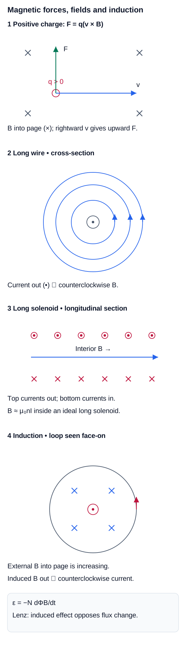
Right-hand-rule magnetic force geometry, circular field around a straight wire, solenoid field, and a loop experiencing changing magnetic flux with induced emf. — Magnetic Force, Field Sources, and Electromagnetic Induction
The panels connect q v cross B force direction, current-produced magnetic fields, and Faraday–Lenz induction from changing magnetic flux.

Direct Current (DC) Circuits

$Resistors in Series and Parallel$

In DC circuits, components can be connected in two primary configurations, which dictate how voltage and current behave across them.

Series Circuits: Components are connected end-to-end, forming a single path. The current ( $I$ ) is identical through all components.
Parallel Circuits: Components are connected across the same two nodes, providing multiple paths. The voltage ( $\Delta V$ ) is identical across all parallel branches.

Equivalent Resistance in Series

Calculates the total resistance of multiple resistors connected in series.

R_{eq} = R_1 + R_2 + R_3 + \dots

Variables

Symbol	Description	Unit
$R_{eq}$	Equivalent series resistance	$\Omega$
$R_i$	Individual resistances	$\Omega$

Equivalent Resistance in Parallel

Calculates the total resistance of multiple resistors connected in parallel.

\frac{1}{R_{eq}} = \frac{1}{R_1} + \frac{1}{R_2} + \frac{1}{R_3} + \dots

Variables

Symbol	Description	Unit
$R_{eq}$	Equivalent parallel resistance	$\Omega$
$R_i$	Individual resistances	$\Omega$

Capacitance and Dielectrics

$Dielectric Materials$

When an insulating material (a dielectric) is placed between the plates of a capacitor, it increases the capacitance of the device by a dimensionless factor called the dielectric constant ( $\kappa$ ).

The molecules in the dielectric become polarized by the external electric field, creating an opposing internal electric field. This reduces the overall electric field between the plates, allowing the capacitor to store more charge for the same applied voltage.

Key Takeaways

Electric Charge is quantized and conserved. Like charges repel, opposites attract according to Coulomb's Law ( $F = kq_1q_2/r^2$ ).
An Electric Field ( $\vec{E} = \vec{F}/q$ ) is created by charges and exerts forces on other charges. Gauss's Law relates flux to enclosed charge.
Electric Potential ( $V = U/q$ ) is energy per unit charge (Voltage). Capacitors ( $C = Q/\Delta V$ ) store charge and energy.
Current ( $I = dq/dt$ ) is the flow of charge, driven by voltage and opposed by Resistance ( $V=IR$ , Ohm's Law).
Moving charges create Magnetic Fields ( $\vec{B}$ ), and magnetic fields exert forces on moving charges ( $\vec{F} = q\vec{v}\times\vec{B}$ ).
A changing magnetic flux induces an EMF (voltage) according to Faraday's Law ( $\mathcal{E} = -d\Phi_B/dt$ ), the basis of electrical generation.

$References$

Previous TopicThermodynamics - Theory & Concepts

Quiz Me

Next TopicOptics and Light - Theory & Concepts

Prev Next

Quiz Me

Learning Objectives

Electric Charge

Electric Charge Concepts

Coulomb's Law

Coulomb's Law Concepts

Coulomb Force Magnitude

Interactive Simulation

The Electric Field (E⃗\vec{E}E)

The Electric Field (E⃗\vec{E}E) Concepts

Electric Field (E⃗\vec{E}E)

Electric Field

Electric Field of a Point Charge

Gauss's Law

Gauss's Law Concepts

Gauss's Law

Electric Potential (VVV)

Electric Potential (VVV) Concepts

Electric Potential (VVV)

Electric Potential

Electric Potential of a Point Charge

Electric Potential (VVV) Concepts

Voltage (Potential Difference)

Capacitance (CCC)

Capacitance (CCC) Concepts

Capacitance (CCC)

Capacitance

Ideal Vacuum Parallel-Plate Capacitor

Capacitance (CCC) Concepts

Current and Resistance

Current and Resistance Concepts

Current (III)

Electric Current

Current and Resistance Concepts

Ohm's Law

Interactive Simulation

Current and Resistance Concepts

Kirchhoff's Rules

Kirchhoff's Rules Concepts

Magnetism

Magnetism Concepts

Magnetic Force (F⃗B\vec{F}_BFB​)

Magnetic Force

Magnetic Force on a Current-Carrying Segment

Work and Magnetic Force

Sources of Magnetic Fields

Sources of Magnetic Fields Concepts

Magnetic Field of a Long Straight Wire

Magnetic Field at the Center of a Circular Loop

Magnetic Field Inside a Long Solenoid

Applications of Magnetism

Electromagnetic Induction

Electromagnetic Induction Concepts

Faraday's Law of Induction

Electromagnetic Induction Concepts

Direct Current (DC) Circuits

Resistors in Series and Parallel

Equivalent Resistance in Series

Equivalent Resistance in Parallel

Capacitance and Dielectrics

Dielectric Materials

References

$Learning Objectives$

$Electric Charge Concepts$

$Coulomb's Law Concepts$

$Interactive Simulation$

The Electric Field ( $\vec{E}$ )

$\vec{E}$

$\vec{E}$

$Gauss's Law Concepts$

Electric Potential ( $V$ )

$V$

$V$

$V$

Capacitance ( $C$ )

$C$

$C$

$C$

$Current and Resistance Concepts$

$I$

$Current and Resistance Concepts$

$Interactive Simulation$

$Current and Resistance Concepts$

$Kirchhoff's Rules Concepts$

$Magnetism Concepts$

$\vec{F}_B$

$Work and Magnetic Force$

$Sources of Magnetic Fields Concepts$

$Applications of Magnetism$

$Electromagnetic Induction Concepts$

$Electromagnetic Induction Concepts$

$Resistors in Series and Parallel$

$Dielectric Materials$

$References$